 Skip to content
AS Level
Mathematics 9709 P1
2. Functions
Written by: Tharun Athreya
Formatted by: Dhyaneshwaran V
Index
2.1 Definition of a function
- A function is a relation that uniquely associates members of one set with the members of another set.
- Functions can also be called mappings.
- Mappings can be:
- ONE-TO-ONE
- MANY-TO-ONE
- ONE-TO-MANY
- MANY-TO-MANY
- Functions can be either a one-one function or a many-one function.
- A one-one function has one output value for each input value.
- A many-one function has one output value for each input value, but each output value can have more than one input value.
- The set of input values for a function is called the domain of the function.
- The set of output values for a function is called the range of the function.
2.2 Composite functions
- When one function is followed by another function, the resulting function is called a composite function.
- \( fg(x) \) means the function \( g \) acts on \( x \) first, then \( f \) acts on the result.
- There are three important points to remember about composite functions:
- \( fg \) only exists if the range of \( g \) is contained within the domain of \( f \).
- In general,
\[ fg(x) \neq gf(x) \] - \( ff(x) \) means you apply the function \( f \) twice.
2.3 Inverse functions
- The inverse function is the opposite of the original function.
- It is denoted by \( f^{-1}(x) \).
- An inverse only exists for one-to-one functions.
- Steps for finding the inverse function:
- STEP-1: Write the function as \( y = f(x) \).
- STEP-2: Interchange the \( x \) and \( y \) variables.
- STEP-3: Rearrange to make \( y \) the subject.
- The inverse function satisfies \( f(f^{-1}(x)) = f^{-1}(f(x)) = x \).
- The domain of \( f^{-1}(x) \) is the range of \( f(x) \).
- The range of \( f^{-1}(x) \) is the domain of \( f(x) \).
- If \( f \) and \( f^{-1} \) are the same function, then \( f \) is called a self-inverse function.
2.4 The graph of a function and its inverse
- The graphs of \( f \) and \( f^{-1} \) are reflections of each other in the line \( y = x \).
- This is because \( f(f^{-1}(x)) = x = f^{-1}(f(x)) \).
- When a function \( f \) is self-inverse, the graph of \( f \) will be symmetrical about the line \( y = x \).
- Example:

2.5 Transformations of functions
Translations
- In translation, the shape, size, and orientation of the graph remain unchanged, but the graph shifts up or down, left or right in the \( xy \) plane.
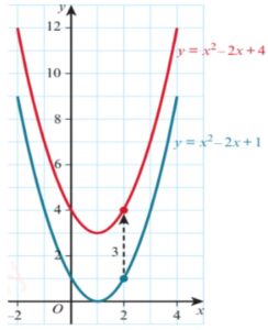
- The graph of \( y = f(x) + a \) is a translation of the graph \( y = f(x) \) by the vector
\[ \begin{bmatrix} 0 \\ a \end{bmatrix} \] - Example:
-
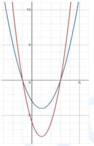
- When the \( x \)-coordinates on the two graphs are the same (\( x = x \)), the \( y \)-coordinates differ by 3 (\( y = y + 3 \)).
- This means that the two curves have exactly the same shape but are separated by 3 units in the positive \( y \)-direction.
- Hence, the graph of \( y = x^2 – 2x + 4 \) is a translation of the graph of \( y = x^2 – 2x + 1 \) by the vector
\[
\begin{bmatrix} 0 \\ 3 \end{bmatrix}
\]
- The graph of \( y = f(x – a) \) is a translation of the graph \( y = f(x) \) by the vector
\[
\begin{bmatrix} a \\ 0 \end{bmatrix}
\] - Example:
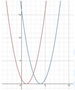
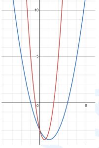
- Equation of the red curve: \( y = x^2 – 2x + 1 \)
Equation of the blue curve: \( y = (x – 3)^2 – 2(x – 3) + 1 \) - The curves have exactly the same shape but are separated by 3 units in the positive \( x \)-direction.
- The \( y \)-coordinates are the same (\( y = y \)), but the \( x \)-coordinates differ by 3 (\( x = x + 3 \)).
- This means that the two curves are at the same height when the blue curve is 3 units to the right of the red curve.
- Hence, the graph of \( y = (x – 3)^2 – 2(x – 3) + 1 \) is a translation of the graph of \( y = x^2 – 2x + 1 \) by the vector
\[
\begin{bmatrix} 3 \\ 0 \end{bmatrix}
\] - Combining these two results gives:
The graph of \( y = f(x – a) + b \) is a translation of the graph \( y = f(x) \) by the vector
\[
\begin{bmatrix} a \\ b \end{bmatrix}
\]
Reflections
- The graph of \( y = -f(x) \) is a reflection of the graph \( y = f(x) \) in the \( x \)-axis.
- Example:
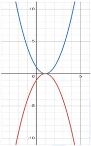
- The equation of the blue curve: \( y = x^2 – 2x + 1 \)
The equation of the red curve: \( y = -(x^2 – 2x + 1) \) - When the \( x \)-coordinates on the two graphs are the same (\( x = x \)), the \( y \)-coordinates are negative of each other (\( y = -y \)).
- This means that, when the \( x \)-coordinates are the same, the red curve is the same vertical distance from the \( x \)-axis as the blue curve but on the opposite side of the \( x \)-axis.
- Hence, the graph of \( y = -(x^2 – 2x + 1) \) is a reflection of the graph of \( y = x^2 – 2x + 1 \) in the \( x \)-axis.
- The graph of \( y = f(-x) \) is a reflection of the graph \( y = f(x) \) in the \( y \)-axis.
- Example:
Stretches
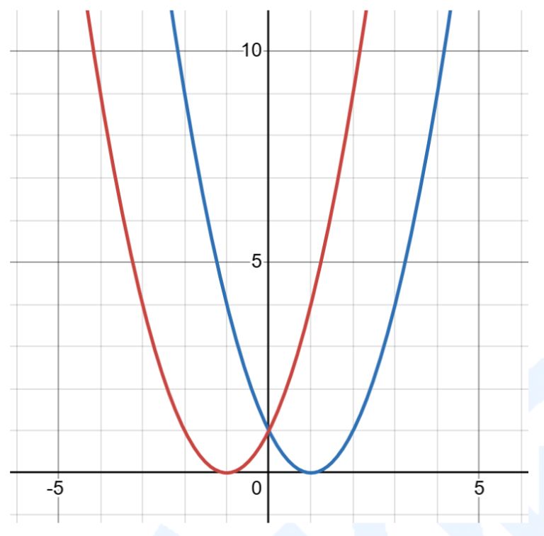
- The graph of \( y = a f(x) \) is a stretch of the graph \( y = f(x) \) with stretch factor \( a \) parallel to the \( y \)-axis.
- Example:
- The equation of the blue curve: \( y = x^2 – 2x – 3 \)
The equation of the red curve: \( y = 2(x^2 – 2x – 3) \) - When the \( x \)-coordinates on the two graphs are the same \((x = x)\),
the \( y \)-coordinate on the red graph is double the \( y \)-coordinate on the blue graph \((y = 2y)\). - This means that, when the \( x \)-coordinates are the same,
the red curve is twice the distance of the blue graph from the \( x \)-axis. - Hence, the graph of \( y = 2(x^2 – 2x – 3) \) is a stretch of the graph of \( y = x^2 – 2x – 3 \)
from the \( x \)-axis. We say that it has been stretched with stretch factor 2 parallel to the \( y \)-axis. - There are alternative ways of expressing this transformation:
- A stretch with scale factor 2 with the line \( y = 0 \) invariant
- A stretch with scale factor 2 with the \( x \)-axis invariant
- A stretch with stretch factor 2 relative to the \( x \)-axis
- A vertical stretch with stretch factor 2.
- Note: if \( a < 0 \), then \( y = a f(x) \) can be considered to be a stretch of \( y = f(x) \)
with a negative scale factor or as a stretch with positive scale factor followed by a reflection in the \( x \)-axis. - The graph of \( y = f(ax) \) is a stretch of the graph \( y = f(x) \)
with stretch factor \( \frac{1}{a} \) parallel to the \( x \)-axis. - Example:
- The equation of the blue curve: \( y = x^2 – 2x – 3 \)
The equation of the red curve: \( y = (2x)^2 – 2(2x) – 3 \) - We obtain the second function by replacing \( x \) by \( 2x \) in the first function.
- The two curves are at the same height \((y = y)\) when \( x = \frac{x}{2} \).
- This means that the heights of the two graphs are the same
when the red graph has half the horizontal displacement from the \( y \)-axis as the blue graph. - Hence, the graph of \( y = (2x)^2 – 2(2x) – 3 \) is a stretch of the graph of \( y = x^2 – 2x – 3 \)
from the \( y \)-axis. We say that it has been stretched with stretch factor \( \frac{1}{2} \) parallel to the \( x \)-axis.
2.6 Combined transformations
- When two vertical transformations or two horizontal transformations are combined, the order in which they are applied may affect the outcome.
- When one horizontal and one vertical transformation are combined, the order in which they are applied does not affect the outcome.
- Vertical transformation follows the ‘normal’ order of operations, as used in arithmetic.
- Horizontal transformations follow the opposite order to the ‘normal’ order of operations, as used in arithmetic.
