 Skip to content
AS Level Physics 9702
1. Physical quantities and units
Written by: Adhulan Rajkamal
Formatted by: Adhulan Rajkamal
Index
1.1 Physical quantities
- All physical quantities → numerical magnitude and a unit
Estimating physical quantities
- Good to know values for estimation:
-
- The resistivity of copper: \(1.68 \times 10^{-8} \, \Omega \text{m}\)
- The Young modulus of steel: \(1.9 \times 10^{11} \, \text{Pa}\)
-
-
For questions involving density → use your knowledge to identify whether the material will float or sink in water; then estimate a density above or below the density of water
-
- Density of water in \(\text{kg m}^{-3}\) → \(1000 \, \text{kg m}^{-3}\)
- Density of water in \(\text{g cm}^{-3}\) → \(1 \, \text{g cm}^{-3}\)
-
- Estimation involves basic real-world knowledge and plugging in reasonable values to equations to derive an estimated calculated value
1.2 SI Units
- SI is founded upon 7 fundamental units known as base units:
| SI Base Quantity | SI Base Unit | Symbol |
|---|---|---|
| Mass | kilogram | kg |
| Length | metre | m |
| Time | second | s |
| Electric current | ampere (amp) | A |
| Temperature | kelvin | K |
| Amount of substance | mole | mol |
| Luminous intensity | candela | cd |
Note: Knowledge about SI base units mole and candela is not required
Derived units
- All quantities other than base quantities → derived quantities
- Derived quantities are expressed using derived units (units derived from the base units)
🔥 Expressing derived units in terms of base units
- All derived units can be expressed in terms of the SI base units from which they are derived.
- Example → Let us express newton (derived unit of force) in terms of the SI base units.
Step 1: State the formula of force
\(F = m \times a\)
Step 2: Express all quantities in the formula in terms of SI base units
\(a = \text{m s}^{-2}\)
\(m = \text{kg}\)
\(F = \text{kg} \times \text{m s}^{-2}\)
| Force expressed in terms of | |
| Derived unit | Base units |
| N | \(\text{kg} \times \text{m s}^{-2}\) |
Therefore, \(N = \text{kg} \times \text{m s}^{-2}\)
Principle of homogeneity
- Principle of homogeneity → In a physical equation, all terms must have the same unit
- Term → individual part of an equation separated by addition (+) or subtraction (−) signs
🔥 Example
Let’s check the homogeneity of the equation:
- \(s = ut + \frac{1}{2} a t^2\)
Step 1: Express all the terms in terms of base units:
\(s \rightarrow \text{m}\)
\(ut \rightarrow (\text{m s}^{-1}) \times \text{s} = \text{m}\)
\(a t^2 \rightarrow (\text{m s}^{-2}) \times \text{s}^2 = \text{m}\)
Note: Constants (e.g., \(\frac{1}{2}\)) can be ignored when dealing with units.
Step 2: Write the formula in terms of the base units:
\(\text{m} = \text{m} + \text{m}\)
Since all terms have the same base units, this satisfies the principle of homogeneity.
- Use the principle of homogeneityin questions asking you to find the unit of a constantin an equation.
Multiples and sub-multiples
| Prefix | Symbol | Multiplying factorial |
|---|---|---|
| Multiples | ||
| tera | T | 1012 |
| giga | G | 109 |
| mega | M | 106 |
| kilo | k | 103 |
| Sub-multiples | ||
| deci | d | 10-1 |
| centi | c | 10-2 |
| milli | m | 10-3 |
| micro | μ | 10-6 |
| nano | n | 10-9 |
| pico | p | 10-12 |
1.3 Errors and uncertainties
- Uncertainty/ Error → Total range of values within which measurements is likely to lie
- All measurements have some level of uncertainty; uncertainty in measurements can be caused by:
- Instrument used
- Method used to take the measurement
- Human error
🔥 The uncertainty value must:
- have the same number of decimal places as the measurement value
- be expressed in one significant figure (1 s.f.)
Absolute Uncertainty
- How to write measurements with uncertainties
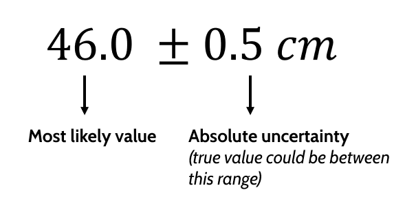
- ⚠️ Note: The measurement and absolute uncertainty must have the same number of decimal places
- Absolute uncertainty is usually 1 sig. fig.
- The absolute uncertainty of an instrument is half its smallest division
- David measured a wire to be 35.5 cm long using a metre rule. Calculate the uncertainty due to the instrument used.
- Smallest division of a metre rule → \(0.1 \, \text{cm}\)
- Half of smallest division → \(\frac{1}{2} \times 0.1 = 0.05 \, \text{cm}\)
- Two measurements are taken:
One at the starting point (where the measurement begins → \(0.0 \, \text{cm}\))
One at the endpoint (where the wire’s length ends → \(35.5 \, \text{cm}\)) - Hence, multiply the uncertainty by 2 → \(2 \times 0.05 = 0.1 \, \text{cm}\)
Percentage uncertainty
- Absolute uncertainty → uncertainty represented in absolute terms
- Percentage uncertainty → uncertainty represented as a percentage of the measurement
🔥 Calculating % uncertainty – example
- David measured a wire to be 35.5 cm long using a metre rule. The absolute uncertainty is 0.1 cm. Calculate the % uncertainty
\(\% \Delta = \frac{\Delta x}{x} \times 100\)
\(= \frac{0.1}{35.5} \times 100\)
\(= 0.28\%\)
\(\text{Hence, measurement is written as } 35.5 \, cm \, \pm \, 0.28\%.\)
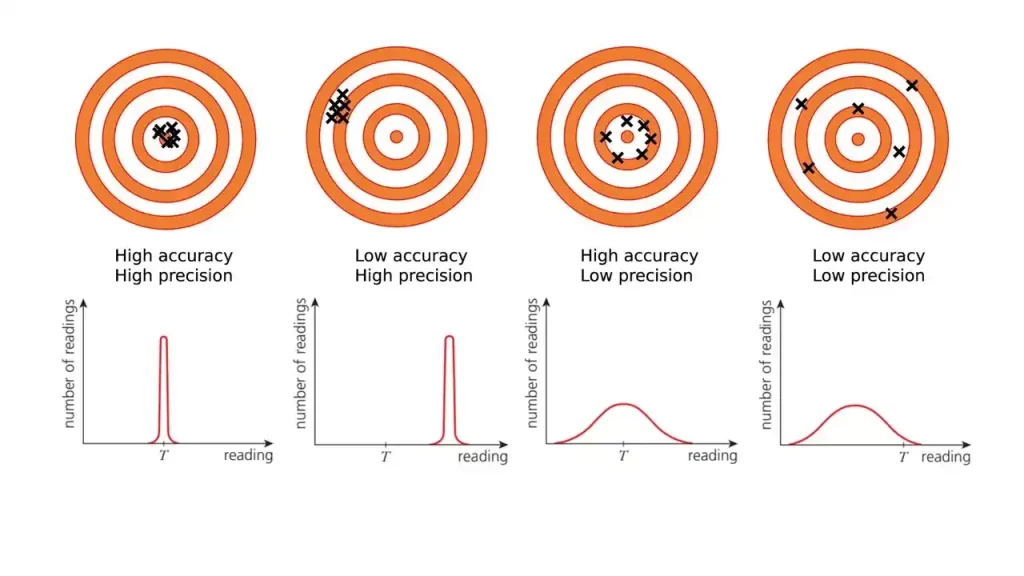
Accuracy and precision
- Accuracy → closeness of a measured value to the ‘true’ or ‘known’ value
- Precision → how close a set of measured values are to each other
Types of errors
| There are two major types of errors | |
|---|---|
| Systematic error | Random error |
| Affects accuracy | Affects precision |
Systematic error
- Causes all readings to deviate consistently (above or below) from the true value
- Fixed Shift: Measurements are offset by a constant amount in the same direction every time
- Cannot be eliminated by repeated readings or averaging
- Can only be minimized by improving experimental techniques
- Reduces the accuracy of measurements
- Examples of systematic uncertainty/error:
- Zero error
- Reading is not zero before measurement
- Wrongly calibrated instrument
- The scale on the instrument may be incorrect
- Reaction time of experimenter
- Usually, there is a delay in starting the timing device after an event has occurred
- Zero error
Random error
- Causes readings to be scattered around the true value
- May be reduced by:
- Repeating a reading and averaging
- Plotting a graph and drawing a best-fit line
- Affects the precision of the measurements
- Examples of random errors:
- Timing oscillations without a reference marker
- Taking readings of a quantity with respect to time → difficulty of reading both time and measurement
- Reading a scale from different angles → parallax error
Combining uncertainties
- Calculating a physical quantity (e.g., speed) requires multiple measurements (e.g., time and distance)
- Each measurement has an associated uncertainty
- The uncertainties must be combined to find the total uncertainty in the calculated quantity
- There are two simple rules for combining uncertainties:
| Quantities are added or subtracted | Quantities are multiplied or divided |
|---|---|
Add absolute uncertainties \( a = b – c + d \) | Add percentage uncertainties \( a = Z \frac{b c}{c} \) Z is a constant – ignored when calculating uncertainty |
- To combine uncertainties for quantities raised to a power, multiply the percentage uncertainty by the power
\( x = \frac{A y^a}{z^b} \quad (A \text{ is constant}) \)
\( \% \Delta x = a (\% \Delta y) + b (\% \Delta z) \)
1.4 Scalars and vectors
- Scalars → Physical quantity which has only magnitude
- Can be added algebraically
- Vectors → Physical quantity with both magnitude and direction
- Cannot be added algebraically
| Scalar quantities | Vector quantities |
|---|---|
| mass | weight |
| speed | velocity |
| energy | acceleration |
| power | force |
| pressure | momentum |
| temperature |
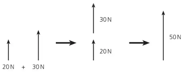
Addition and subtraction of coplanar vectors
- Coplanar vectors → Vectors that lie in the same plane
- Adding two vector quantities is not straightforward since direction both direction and magnitude is present
- Addition of coplanar vectors:
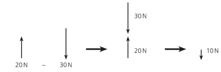
- Subtraction of coplanar vectors:
Addition of non-planar vectors
- Where vectors are not coplanar → resultant vector is found by using a vector triangle
- Vector triangle example:

- Connect the head of a vector the tail of another
- Draw a line from the tail of the first vector to the head of the final vector → this is the resultant vector
Resolving vectors
- 2 vectors may be added to produce a single resultant vector
- Resolving vectors → one vector split into two perpendicular components (opposite of previous statement)
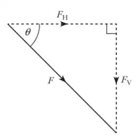
- Consider the vector as the hypotenuse of a right triangle
- Draw the other two sides of the triangle
- Ensure the sides are perpendicular to each other
- To calculate the magnitude of the each of the two components of a vector use trigonometric functions
- \(F_H = F \cos\theta\) → magnitude of horizontal component
- \(F_V = F \sin\theta\) → magnitude of vertical component
(Refers to the previous diagram)
